I recently had this thought that there are two kinds of scientists, or at least two different approaches to getting into science. We either want to understand the world, or we want to change the world.
This is a frequent contention in refereeing both articles and grants. Some will ask you in what way you are describing a new phenomenon or mechanism, while others will ask how your results are likely to change the world.
Physiology is by nature more of a science that tries to understand the world.
Clinical trials is the archetype of science that tries to change the world.
It is by no means necessary to understand the world in order to change it. A true trialist will answer the question of how does your intervention work with a disdainful: "I don't care".
The same goes for the risk factors identified in epidemiological research. They are risk factors because they are associated with some deleterious outcome, not because they are causal, or because we know how it works.
So, the question arises. Why do you do your science?
Saturday, April 13, 2019


Angiotensin II and allostasis
Recently, we talked about allostasis, which is an extension of classical homeostatic regulation to include neural and hormonal signals that can reset homeostatic set points to anticipate changes in the environment.
As I was preparing to submit an abstract to Experimental Biology, which is the major conference in physiology, I realised that a paper that we published recently includes a potential example of allostatic regulation.
It turns out that the hormone angiotensin II that works to retain sodium and increase blood pressure also leads to increased production of the transcription factor NFAT5. This would be allostatic because when the kidney retains sodium the amount of sodium in the interstitial fluid in the medulla of the kidney increases, which means that its tonicity (the number of molecules per volume fluid) also increases and in turn causes osmotic stress. Normally, NFAT5 that is also known as Tonicity-responsive enhancer binding protein (TonEBP) reacts to changes in tonicity to activate genes that protect the cells. In this setting, it appears that the cells can anticipate increased tonicity by sensing angiotensin II directly and increasing the production of NFAT5 to be better prepared to respond to the change in osmotic stress that will come as an effect of the increased angiotensin II concentration.
I was happy to have the abstract well-received and actually got a talk, as well as a fair bit of interest at the poster.
As I was preparing to submit an abstract to Experimental Biology, which is the major conference in physiology, I realised that a paper that we published recently includes a potential example of allostatic regulation.
It turns out that the hormone angiotensin II that works to retain sodium and increase blood pressure also leads to increased production of the transcription factor NFAT5. This would be allostatic because when the kidney retains sodium the amount of sodium in the interstitial fluid in the medulla of the kidney increases, which means that its tonicity (the number of molecules per volume fluid) also increases and in turn causes osmotic stress. Normally, NFAT5 that is also known as Tonicity-responsive enhancer binding protein (TonEBP) reacts to changes in tonicity to activate genes that protect the cells. In this setting, it appears that the cells can anticipate increased tonicity by sensing angiotensin II directly and increasing the production of NFAT5 to be better prepared to respond to the change in osmotic stress that will come as an effect of the increased angiotensin II concentration.
I was happy to have the abstract well-received and actually got a talk, as well as a fair bit of interest at the poster.
Wednesday, November 21, 2018
Maintaining homeostasis by prophecy
Homeostasis is the idea of an ideal internal milieu for the cells that the body strives to maintain. The idea was initially proposed by Walter B. Cannon and remains a central tenet of physiology. One of the most basic regulatory mechanisms used to achieve this is negative feedback, wherein a change in some important parameter triggers a compensatory response that serves to bring it back toward the optimal level. This entails that for any true homeostatic parameter there should be an ideal set point. However, there are many such systems that will reset the regulation of their parameter either in response to outside stress, or in disease. Many, if not most researchers have had no problem with expanding the remit of homeostatic regulation to include resetting and learnt neurohormonal mechanisms that might anticipate an environmental challenge. But others felt the need to come up with new words to encapsulate these parts of physiological regulation.
One attempt to conceptualise this is the idea of allostasis, or achieving stability through change. Either change in the set point of a parameter, or change in behaviour, and that this could even be done in anticipation of a change in environment. This is different from the classical view of homeostasis where the organism reacts to a change in a critical parameter and strives to return it to normal. However, allostasis is still poorly defined and researchers that use the term do not agree completely what it means. Some see it as an extension of normal homeostatic physiology, others see allostasis as a pathological process. When you see it as pathological it makes sense to talk about the extra energy expended to change and maintain a homeostatic set point at a new level, or the extra energy expended to perform a changed behaviour. To describe this the researchers who see allostasis as pathological use the term allostatic load, or allostatic stress.
Anyway, if we return to the perspective of the cells with a speculative example; A kidney cell cannot sense a change in outside temperature that will lead to increased metabolic rate, that will lead to increased protein intake, that will lead to increased urea production, that will require increased glomerular filtration in the kidney. So, it has developed a brain and a skin with temperature sensors that tells the brain that it is colder out isde. The brain can then tell cells that produce heat to produce more heat to maintain body temperature. The brain can potentially also tell the kidney that it is making the heating cells work harder and thus that glomerular filtration will need to increase in the near future. While, this example is mostly speculation it serves as an example of a mechanism that would be difficult to fit into a classical homeostatic mechanism. Thereby, it illustrates the usefulness of a new concept whereby a kidney cell could develop a prophetic (for other kidney cells) ability to foresee the need increased work in the future.
One attempt to conceptualise this is the idea of allostasis, or achieving stability through change. Either change in the set point of a parameter, or change in behaviour, and that this could even be done in anticipation of a change in environment. This is different from the classical view of homeostasis where the organism reacts to a change in a critical parameter and strives to return it to normal. However, allostasis is still poorly defined and researchers that use the term do not agree completely what it means. Some see it as an extension of normal homeostatic physiology, others see allostasis as a pathological process. When you see it as pathological it makes sense to talk about the extra energy expended to change and maintain a homeostatic set point at a new level, or the extra energy expended to perform a changed behaviour. To describe this the researchers who see allostasis as pathological use the term allostatic load, or allostatic stress.
Anyway, if we return to the perspective of the cells with a speculative example; A kidney cell cannot sense a change in outside temperature that will lead to increased metabolic rate, that will lead to increased protein intake, that will lead to increased urea production, that will require increased glomerular filtration in the kidney. So, it has developed a brain and a skin with temperature sensors that tells the brain that it is colder out isde. The brain can then tell cells that produce heat to produce more heat to maintain body temperature. The brain can potentially also tell the kidney that it is making the heating cells work harder and thus that glomerular filtration will need to increase in the near future. While, this example is mostly speculation it serves as an example of a mechanism that would be difficult to fit into a classical homeostatic mechanism. Thereby, it illustrates the usefulness of a new concept whereby a kidney cell could develop a prophetic (for other kidney cells) ability to foresee the need increased work in the future.
Wednesday, October 17, 2018
Cell death used to be easy
I was recently happy to be asked to write a chapter about cell death in the new version of the Swedish textbook on intensive care medicine (You'll find the previous edition here we expect the new one to be published in 2019). Touching up on cell death i found this paper where the leaders everyone in the field spell out the latest understanding about different forms of regulated cell death.
When I last read about cell death it was recognised that there were two basic types, necrosis, that is normal cell death, and apoptosis or programmed cell death. I had heard a little about necroptosis, as it was recently shown to be important in the kidney. I also recognised the name autophagy, but rather thought it was something liver cells did in starvation. It still does, but now it is also a general term for a kind of cell death machinery as well.
It turns out there are now twelve types of regulated cell death (RCD), and even the morphology is no longer any indication of the type of cell death involved. Because, as they write,
On the other hand, the great number of different mechanisms opens the possibility of an equally great number of new and shiny papers.
When I last read about cell death it was recognised that there were two basic types, necrosis, that is normal cell death, and apoptosis or programmed cell death. I had heard a little about necroptosis, as it was recently shown to be important in the kidney. I also recognised the name autophagy, but rather thought it was something liver cells did in starvation. It still does, but now it is also a general term for a kind of cell death machinery as well.
It turns out there are now twelve types of regulated cell death (RCD), and even the morphology is no longer any indication of the type of cell death involved. Because, as they write,
"Moreover, each type of RCD can manifest with an entire spectrum of morphological features ranging from fully necrotic to fully apoptotic, and an immunomodulatory profile ranging from anti-inflammatory and tolerogenic to pro-inflammatory and immunogenic."This plethora of mechanisms does rather complicate the understanding of cell death. Especially so as most of the mechanisms can be activated a little bit and then regress, as long as the death threshold has not been reached. And, even more so as they may switch mechanism if you try to intervene against one of the pathways. This is actually one of the major take-home messages of the paper. We have tried a number of different cell death inhibitors that seem to work in experimental systems where the trigger is controlled. However, when we try them out in patients we find that the cells die anyway.
On the other hand, the great number of different mechanisms opens the possibility of an equally great number of new and shiny papers.
Tuesday, October 16, 2018
Monitoring in anaesthesia and intensive care - 8th Hedenstierna symposium
Activity has not been the highest as of late, but now I am back (perhaps anyway). Today I attended the Hedenstierna symposium in Uppsala on the actual 77th birthday of Göran Hedenstierna himself. He attended, as he always does, and he was suitably embarrassed when the whole meeting sang happy birthday to him.
The good thing with having a famous scientist to name your seminar after is that you can attract real top-names from around the world. This means there are ample opportunities to expand your network both in your field and in associated fields. There were the brilliant Göran Stemme, group leader from KTH who developed the microneedles me and his former student Niclas Roxhed wrote about some years ago. Then Michell Chew chewed on about the very current area of using point-of-care ultrasound in intensive care, and Fernando Sipmann simpered (not really) on monitoring the respiration. After lunch, Declan Bates declared a sermon on mathematical modelling that none of us really understood, but it was very impressive. Finally, Marlies Ostermann orated about the actually important organs, the kidneys. She had a hard time convincing the mostly respiratory scientists in the audience that kidneys are quite simple and just the most fun to be had in physiology.
It wasn't really the final talk, there were Johanna Hästbacka from Helsinki who talked on monitoring inflammation, and Emory Brown from America on neuromonitoring, but I had to pick up my dog from daycare and missed out.
The good thing with having a famous scientist to name your seminar after is that you can attract real top-names from around the world. This means there are ample opportunities to expand your network both in your field and in associated fields. There were the brilliant Göran Stemme, group leader from KTH who developed the microneedles me and his former student Niclas Roxhed wrote about some years ago. Then Michell Chew chewed on about the very current area of using point-of-care ultrasound in intensive care, and Fernando Sipmann simpered (not really) on monitoring the respiration. After lunch, Declan Bates declared a sermon on mathematical modelling that none of us really understood, but it was very impressive. Finally, Marlies Ostermann orated about the actually important organs, the kidneys. She had a hard time convincing the mostly respiratory scientists in the audience that kidneys are quite simple and just the most fun to be had in physiology.
It wasn't really the final talk, there were Johanna Hästbacka from Helsinki who talked on monitoring inflammation, and Emory Brown from America on neuromonitoring, but I had to pick up my dog from daycare and missed out.
Saturday, August 04, 2018
Print mounting
I am on vacation and finally had a bit of time to mount some of my prints, which I am going to hang in my home office. The home office is rather more important as the hospital has decided to remove our offices because there are workplaces at the operating and intensive care departments. That any doctor would have "stuff" or "papers" is apparently nonsensical. The patient data management system is digital now, and thus we do not need papers, and do not need a personal space.
Anyway, mounting prints is almost as much of a discussion point in photography as all the other things. I learnt how I do it from a Luminous Landscape tutorial, but since I mostly mount smaller prints I eschew hinging the mats, and mostly only mount with mounting corners. We will see.

First and foremost we knoll, as we learnt from Adam Savage through Tested.com. We have four prints and five sets of frames, backs and mats. So, we'll have to find a final print somewhere. When we haven't decided which prints to mount it is an idea to get symmetric mats so that we can decide which whether to use portrait or landscape orientation later. If we know which print we will mount, then slightly asymmetric mats with a thicker lower edge is often more elegant. Let's start with the elephant.


The frames are Nielsen aluminium profile frames that we put together with these simple corner fixtures consisting of a right-angle plate with two set screws and a shim to distribute the force on the aluminium. In addition there are two hanging fixtures to slide in, and fasten with set screws. For now we will leave one side unmounted to be able to get the print in.


Before sliding the mounted print in, we peel the cover off of the plexiglass and place it on the matted picture and make very sure there is no dust in between. A simple dust blower makes short work of any dirt. By now we really should have signed the mats if we wanted to do that.


Anyway, mounting prints is almost as much of a discussion point in photography as all the other things. I learnt how I do it from a Luminous Landscape tutorial, but since I mostly mount smaller prints I eschew hinging the mats, and mostly only mount with mounting corners. We will see.


Step one is to place the print and fit the mat. An important point is that it shouldn't move until it is fixed in place, for that purpose we use a weight. A, flat, clean and heavy weight.


With the weight in place we then place the mounting corners. Since these are small A4-size images, they will stay in place using just corners and the mat. Once the picture is securely mounted, we need to double-check that it fits the mat so that we don't find any mistakes after we mount it.


Before sliding the mounted print in, we peel the cover off of the plexiglass and place it on the matted picture and make very sure there is no dust in between. A simple dust blower makes short work of any dirt. By now we really should have signed the mats if we wanted to do that.


In order to keep the stack of backing, print, mat and glass in place the Nielsen system uses leaf springs that you push in under the edges of the frame. I tend to use two per side for A4-size prints.


The last step is to put some hanging wire in place. By only twisting one side to start with it is easy to regulate the height when we actually hang the prints. Oh, and that's one, now for the other four, whereof one needs to be selected and printed first.

But, after all that I have more of my own art on the walls, which is nice. Thank you for following along.
Monday, July 18, 2016
What makes a scientist?
@RealScientists is a scientific outreach Twitter-account that invites a new scientist to talk about their research every week. It is good fun and often very interesting including everything from actual details of data collection in botany and astronomy, to work/family-balance and career planning. Recently, @drclairemurray curated the account and asked the question:
From this perspective I would like to argue that scientists are like football players. As long as they continue pursuing their own original research and publish with peer-review as the lead or senior author they are still scientists. This is a high bar, and there are some points in this argument that warrant a bit of an explanation.
1: "continue pursuing" means that as soon as they quit actively doing research they also stop being scientists.
2: "their own" means that if they don't provide substantial intellectual input to coming up with the idea, designing and performing the work, and interpreting the results it does not count. This does not mean it has to be only theirs with no outside input, which would be silly.
3: "original research" means that it should be providing either new data, or new interpretations. Experimental reproduction counts, pure theory too, even meta analysis is alright.
4: "publish with peer-review" means just that. The results have to be double-checked by experts and have to be made available to everyone else both now and in the future through publication. This can mean that a bachelor thesis is an adequate start.
5: "lead or senior author" means that they should be the driving force behind publication. The actual position in the author list is not important for the argument, although it is very telling in a field like medicine.
We should, however, be aware that there is an argument for setting the bar low. If they get to identify as scientists already when they do their first experiment and continue to as long as they think rationally, maybe it would be easier to recruit new researchers; maybe the anti-science attitude in the society would decrease; maybe rational thought would be hip again.
Which was followed by a barrage of answers. Most of which wanted to set the bar really low so that curiosity alone would be a sufficient characteristic. I would rather we set a higher standard so that scientist is something you can strive to become, and have to strive to remain (although often I would like it to be easier).Sunday is the perfect time to get philosophical, right? I wonder what you think makes a scientist?— realscientists (@realscientists) July 17, 2016
From this perspective I would like to argue that scientists are like football players. As long as they continue pursuing their own original research and publish with peer-review as the lead or senior author they are still scientists. This is a high bar, and there are some points in this argument that warrant a bit of an explanation.
1: "continue pursuing" means that as soon as they quit actively doing research they also stop being scientists.
2: "their own" means that if they don't provide substantial intellectual input to coming up with the idea, designing and performing the work, and interpreting the results it does not count. This does not mean it has to be only theirs with no outside input, which would be silly.
3: "original research" means that it should be providing either new data, or new interpretations. Experimental reproduction counts, pure theory too, even meta analysis is alright.
4: "publish with peer-review" means just that. The results have to be double-checked by experts and have to be made available to everyone else both now and in the future through publication. This can mean that a bachelor thesis is an adequate start.
5: "lead or senior author" means that they should be the driving force behind publication. The actual position in the author list is not important for the argument, although it is very telling in a field like medicine.
We should, however, be aware that there is an argument for setting the bar low. If they get to identify as scientists already when they do their first experiment and continue to as long as they think rationally, maybe it would be easier to recruit new researchers; maybe the anti-science attitude in the society would decrease; maybe rational thought would be hip again.
Wednesday, June 29, 2016
Widefield astrophotography setup


The autoguider is mounted on an accessory bracket with a block for mounting on photographic tripods that has a standard tripod mounting hole on the bottom. The bracket and mounting block came with the telescope. Then we can just screw the camera and guider to either side of a standard Vixen dovetail bar. Finally we mount all of that ontop of a computer-controlled Sky-Watcher HEQ5 because: Stability!

Transit of Mercury 2016-05-09

The transit of Mercury happened! Luckily I could escape a little bit early on transit day and set up the telescope to catch us a transit. We see that the gear is a fairly basic set up based on a Sky-Watcher ED80 equipped with a neutral density photographic solar filter from Baader Planetarium and a Canon D600.


In the end I got a little bit sunburned and Skrållan, my then 9-week-old boxer puppy, found a bit of shade by the photo bag.

We saw the whole picture at the top of the page with Mercury to the left and a couple of sunspots in the middle. Below we see two 100% close-up cropped frames to get a better look at the details. The difference between sunspots that are irregular and are surrounded by a lighter penumbra, and the silhouette of Mercury that is perfectly (to the limit of the camera) round and smooth is easy to see.


Saturday, June 11, 2016
Some nebulosities in Orion
Orion is one of the most spectacular parts of the sky with enormous, extended nebulas, including the brightest nebula in the northern sky. The aptly named Great nebula in Orion, often known as the Orion nebula, but we will leave that for another time and focus on two other bright and well-known nebulae.


To set the scene we start with a wide field image from a true dark-sky site at 4000m in northern India. It is only a single frame with about 30s exposure. But there is so little light pollution that it is actually hard to pick out the constellations among all the stars.

Anyway, here are the major stars in Orion. As we see they have mostly old arabic names, which is where most historical knowledge of the stars come from. Admittedly, from astrology, but at least they tried.

Now we will turn our attention to two of the nebulae to have a closer look. The Flame nebula, NGC2024, and the very well-known Horsehead nebula IC434.

First we switch from an 11.5 mm aperture f2 camera lens to a proper telescope. In this case a 106 mm f5 Takahashi FSQ ED at iTelescope's observatory at Siding Spring Observatory, Australia. It is located just by the 4-meter Anglo-Australian Telescope. It gives a nice view that includes both nebulae.

Then, we can switch to the 700mm BCL telescope, named for Dame Jocelyn Bell Burnell, Annie Jump Cannon and Henrietta Swan Leavitt, which is a beast among amateur equipment. This gives us a real close-up view of the Horse Head Nebula, which is where we leave off for today.


Anyway, here are the major stars in Orion. As we see they have mostly old arabic names, which is where most historical knowledge of the stars come from. Admittedly, from astrology, but at least they tried.

Now we will turn our attention to two of the nebulae to have a closer look. The Flame nebula, NGC2024, and the very well-known Horsehead nebula IC434.

First we switch from an 11.5 mm aperture f2 camera lens to a proper telescope. In this case a 106 mm f5 Takahashi FSQ ED at iTelescope's observatory at Siding Spring Observatory, Australia. It is located just by the 4-meter Anglo-Australian Telescope. It gives a nice view that includes both nebulae.
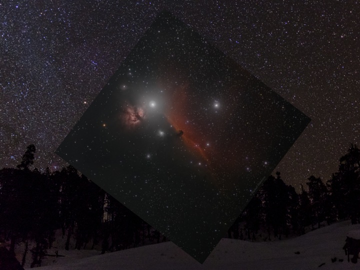
Then, we can switch to the 700mm BCL telescope, named for Dame Jocelyn Bell Burnell, Annie Jump Cannon and Henrietta Swan Leavitt, which is a beast among amateur equipment. This gives us a real close-up view of the Horse Head Nebula, which is where we leave off for today.

Sunday, October 04, 2015
Astronephrologist
 |
| Dumb bell nebula, M27. |
Eventually I decided on a telescope, or three, but today we'll discuss learning proper astrophysics online. While surfing around I came across these wonderful astronomy courses on edX.org given by Paul Francis and Brian Schmidt at the Australian National University. There are four courses: Greatest unsolved mysteries of the universe, Exploring exoplanets, The violent universe, and Cosmology. Together they correspond to ANU's first year of astrophysics. If you would like to start a bit more basic there's also the Introduction to solar systems astronomy given by Frank Timmes at Arizona State University.
Genetics and medicine has little compared to astronomy when it comes to data availability. It turns out that most catalogues of stars, galaxies, etc. get turned into public databases fairly quickly, which is reasonable given the small number of really large telescopes and space missions compared to the amount of data one of these can collect (Oh, and the number of undergrads astrophysics departments around the world have to contend with). So, I downloaded the Hipparcos and Tycho2 catalogues and played around with them in R. Good fun for summer vacation. I might write a bit more about that later. Here's a star density plot of the Tycho2 data for now.
 |
| Tycho2 star density in a galactic aitoff projection produced using R. We can clearly see the dust clouds that obscure parts of the galaxy from view. |
Wednesday, April 08, 2015
A more reasonable look at exercise guidelines
We are going to revisit the exercise guidelines because there is a new meta analysis in JAMA of Leisure Time Physical Activity and Mortality: A Detailed Pooled Analysis of the Dose-Response Relationship that tries to answer the question of how much training is optimal in a more precise way. As we discussed previously, the official exercise recommendations can be hard to understand from an amateur or elite athlete's perspective. Training at that level is not focused on health benefits per se, but on improving performance. The problem lies in the rough dichotomies for both time and intensity in the guidelines. For example:
The first problem we will tackle is the amount of exercise. The best way of measuring physical activity is using prospective logging. That is, each participant maintains a detailed log of all activities, usually for a week. This measure corresponds well with energy expenditure measured using doubly labelled water. However, for the kind of large epidemiological studies used to base the exercise guidelines on that is too much work. Instead they rely on seven-day recall questionnaires, which basically means asking the participants what they did last week hour by hour. This is a poor estimate of actual exercise but an acceptable measure for comparing different groups of people or the same people at different time points. As expected people tend to over estimate their physical activity using the recall method. One study found an average under estimation of 40% for total duration of exercise but a massive four-fold over estimation of vigorous exercise using recall instead of logs. The result was a 70% over-estimate of exercise amount when corrected for intensity. In addition, being part of a study means that logged exercise will probably be larger than exercise during an average non-logged week. Importantly, any of the methods will probably over estimate the average amount of exercise compared to a long-term exercise log, which includes vacations, injuries, and general laziness. Anyway, this is an important part of the reason why the guidelines basically give two intervals for training amount: Less than 150 minutes/week is bad for you, and more than 150 minutes/week is good for you.
Our second scab to pick is the intensity, which is dichotomised to moderate or vigorous both in the guidelines and in the original publications. Moderate is walking or bicycling in a brisk pace, but not strenuously. Vigorously is anything more intensive than walking or bicycling, for example jogging or swimming. Behind this artificial dichotomy lies the actual activities and in research about physical activity the intensity of different forms of exercise is quantified in metabolic equivalents or METs. The number of METs that an activity has is determined by how many times the resting energy expenditure the activity consumes. Using the kind of exercise and the number of hours we can then calculate an amount of exercise corrected for intensity. This is called MET-hours, that is the number of hours of exercise at a given MET-intensity. The minimum exercise in the guidelines correspond to 7.5 MET-hours per week, and the higher goal for additional benefits is accordingly 15 MET-hours/week.
Using the Compendium of physical activities we can calculate how many MET-hours my training actually corresponds to. Judo has a MET of 10 and weightlifting 6. This works out to 22 MET-hours Judo and 3 MET-hours strengthening for a total of 25 MET-hours, which is satisfyingly above the goal for maximum benefit.
Finally, we can get back to the new analysis. What they did was go back to the original data and use the MET-hours recorded for each participant at leisure-time physical activity (i.e. exercise). This was then compared to the risk of death for different amounts of intensity corrected exercise. In figure 1 we can see that we can lower our risk of death by up to 40% by training more than 22 MET-hours per week and less than 75 MET-hours per week. However, we also see that the dichotomy holds. If we train at least 7.5 MET-hours per week we get the bulk of the benefit.
We can conclude that how long we, or our patients, should train depends very much on the type of training. When using these guidelines, even with correction for type of training, we should remember that they are based on reducing the risk of death. They are not meant to help you improve performance, certainly not at the serious amateur or elite level. Finally, while we can understand the reasoning behind making the guidelines as easy as possible, it would be useful to explain how to grade different forms of exercise quite early in the actual guidelines instead of leaving it to the reader to find in original sources.
"Adults aged 18–64 should do at least 150 minutes of moderate-intensity aerobic physical activity throughout the week or do at least 75 minutes of vigorous-intensity aerobic physical activity throughout the week" (WHO exercise guidelines 2010)In my previous post we saw that I managed 164 minutes per week on average over a two year period including about 20% strengthening that should be counted separately. If we work that out, it is about 132 minutes aerobic training (mostly judo) and 32 minutes strength training per week. That is enough exercise if we count judo as a vigorous activity, which seems reasonable. However, we note that it does not reach the optimum of 300 minutes of moderate-intensity or 150 minutes of vigorous-intensity exercise plus two sessions of strength training per week. At the same time it is at the top level of recreational judo. So, something is not quite right.
The first problem we will tackle is the amount of exercise. The best way of measuring physical activity is using prospective logging. That is, each participant maintains a detailed log of all activities, usually for a week. This measure corresponds well with energy expenditure measured using doubly labelled water. However, for the kind of large epidemiological studies used to base the exercise guidelines on that is too much work. Instead they rely on seven-day recall questionnaires, which basically means asking the participants what they did last week hour by hour. This is a poor estimate of actual exercise but an acceptable measure for comparing different groups of people or the same people at different time points. As expected people tend to over estimate their physical activity using the recall method. One study found an average under estimation of 40% for total duration of exercise but a massive four-fold over estimation of vigorous exercise using recall instead of logs. The result was a 70% over-estimate of exercise amount when corrected for intensity. In addition, being part of a study means that logged exercise will probably be larger than exercise during an average non-logged week. Importantly, any of the methods will probably over estimate the average amount of exercise compared to a long-term exercise log, which includes vacations, injuries, and general laziness. Anyway, this is an important part of the reason why the guidelines basically give two intervals for training amount: Less than 150 minutes/week is bad for you, and more than 150 minutes/week is good for you.
Our second scab to pick is the intensity, which is dichotomised to moderate or vigorous both in the guidelines and in the original publications. Moderate is walking or bicycling in a brisk pace, but not strenuously. Vigorously is anything more intensive than walking or bicycling, for example jogging or swimming. Behind this artificial dichotomy lies the actual activities and in research about physical activity the intensity of different forms of exercise is quantified in metabolic equivalents or METs. The number of METs that an activity has is determined by how many times the resting energy expenditure the activity consumes. Using the kind of exercise and the number of hours we can then calculate an amount of exercise corrected for intensity. This is called MET-hours, that is the number of hours of exercise at a given MET-intensity. The minimum exercise in the guidelines correspond to 7.5 MET-hours per week, and the higher goal for additional benefits is accordingly 15 MET-hours/week.
Using the Compendium of physical activities we can calculate how many MET-hours my training actually corresponds to. Judo has a MET of 10 and weightlifting 6. This works out to 22 MET-hours Judo and 3 MET-hours strengthening for a total of 25 MET-hours, which is satisfyingly above the goal for maximum benefit.
 |
| Figure 1 adapted from Leisure Time Physical Activity and Mortality: A Detailed Pooled Analysis of the Dose-Response Relationship by Hannah Arem and co-workers, JAMA Internal Medicine 6 Apr 2015. |
We can conclude that how long we, or our patients, should train depends very much on the type of training. When using these guidelines, even with correction for type of training, we should remember that they are based on reducing the risk of death. They are not meant to help you improve performance, certainly not at the serious amateur or elite level. Finally, while we can understand the reasoning behind making the guidelines as easy as possible, it would be useful to explain how to grade different forms of exercise quite early in the actual guidelines instead of leaving it to the reader to find in original sources.
Saturday, March 07, 2015
Meta analysis in R
or
the beneficial effect of teaching on research
I have been fascinated by meta analysis for a long time. It is so obviously the right way to approach the true effect of an intervention. Recently, an old binder presented itself in aWhich brings us to the the story I am about to tell. Four or five years ago, when I moved back to Uppsala, I got offered a lecture on physiological changes in the elderly. It was to be part of a final year course for the master in biomedicine programme. Just a single hour to show how all the physiology from the rest of the programme changed with age. To compare and contrast ageing as such with the accrued ailments of living for a long time, and distinguish these from the chronic and age related disease. It was not a huge success, but given the title I was not too disillusioned. The second year I was given two hours. Still a bit on the short side, but one hundred percent better than one.
It is not the most popular lecture, but I have had it for five years now and one of the things I teach is that some parts of ageing is caused by metabolism itself. The burning of oxygen singes the organism and with time it will break much like the paneling in an old sauna. As proof of this I used the idea of caloric restriction, which can prolong life in many strains of yeast, mice, and rats. Then, in 2012 an article was published on the effect of caloric restriction in the Rhesus monkey, a primate, and reasonably the closest relative to humans in which an experiment could be expected to be finished any time soon. It showed no effect. I happily included this in my lecture as a counter-point. Until in 2014, when updating the lecture for a new semester, I found that another experiment with caloric restriction in Rhesus monkeys had published their data and found a clear difference.
This made it hard to continue the lecture as I had done, I could just show both studies and say that we don't know. But the total number of animals included was quite large, and the effect measure very straight-forward. Death. So, I performed a meta analysis of mortality of these two studies, and a third smaller study published in 2003. This is the story of that analysis.
Quickly I installed the R package rmeta by Thomas Lumley and set to work. It is quite easy really, we start with setting up a table of results from the included studies. The table should include the total number of subjects in each group, and the number of deaths per group.
 |
| Hultström, M. Acta Physiol (Oxf). 2015 Feb 14. doi: 10.1111/apha.12468. |
 |
| Hultström, M. Acta Physiol (Oxf). 2015 Feb 14. doi: 10.1111/apha.12468. |
There was no significant effect of caloric restriction on all cause mortality in Rhesus monkeys. Or, rather there was a small, clearly non-significant, effect. One of the reviewers asked what would be needed to show if this effect was true. That is, could I please perform a power analysis. So, I installed the pwr package and ran a 2p2n.test() using the most generous effect estimate, i.e. a hypothetical study that ran to completion where the whole control population had died giving an effect of 0.08. This resulted in a required population of 2806 subjects to reach 85% power. This is the power-level which is normally used as the basis for power calculation in clinical studies. However, the age-related mortality was a different story that you can find in the actual article.
The next thing that surprised me was how difficult it was to get this simple little analysis published. It appears that experimental journals don't publish meta analyses, and clinical journals that publish meta analyses, don't publish experimental results. Finally, I found a benevolent editor at Acta Physiologica who permitted it to be published as an editorial. So that is where it resides today, and finally I can give a fairly clear answer in my lecture on the effect of reducing metabolism by caloric restriction on ageing and on mortality. Only problem is, I now have to explain meta analysis and forest plots before I can show the actual data.
And, no I am not going to starve myself so that I can avoid some diseases we can treat in favour for a frailty for which the only known treatment is eating more.
And, no I am not going to starve myself so that I can avoid some diseases we can treat in favour for a frailty for which the only known treatment is eating more.
Sunday, January 04, 2015
Fujifilm X100T first impressions

1. The burst mode does not lock the camera so it is possible to take another burst almost directly.
2. There is a setting for release priority, and it is separate for continuous and single shot focus so that you can have one for each.
3. There is no tab on the focus wheel, nor is there always-on manual focus. However, the manual focus is excellent with split-screen, peaking, and 100%-preview modes.
4, 6, 7, & 8. While there are no dedicated switches, there is a drive-mode button for selecting single, continuous, bracketing, or film mode, and there are seven programmable buttons that I have programmed to cover my needs.
5. There is no dedicated ISO dial. Although, I have high hopes for a firmware update that lets you use the exposure-compensation dial for ISO. It should be easy, really.
9. While there is no touch screen, the buttons are much better with a dedicated back button to get out of menus.As you see, it still does not have a manual ISO dial, but otherwise I am happy. It is a massive improvement above the X100, which, given how much I liked the X100, is no idle praise. The film simulation is particularly useful when working in black and white, I have the camera set that way and have Adobe Lightroom set up to import as low-contrast black and white. It works excellently. High ISO is excellent up to 6400. I haven't had use for higher ISO seeing as I am only in Sweden in January, and not in a mine. Macro shooting also works well, at f2 the actual focus seems to lie slightly in front of the apparent focus using peaking manual focus, and autofocus is not the most accurate. Honestly, f2, autofocus, and macro are three things that don't generally go together. So, I can't really fault the camera for that.
Here are some examples from the first days of shooting. As you see it works right out of the box for boxer snaps.

With a little bit of thought it can take quite nice portraits.

And night-time shooting at ISO 6400 is no problem and gives very presentable result.


Sunday, December 28, 2014
Your move, Fujifilm!
This is what I have:

This is what I want:
 And the page to do it is already there:

Please, please, pretty please, upgrade the X100T so that ISO can be controlled with the exposure compensation dial!
This is what I want:
Please, please, pretty please, upgrade the X100T so that ISO can be controlled with the exposure compensation dial!
Wednesday, November 26, 2014
Tag clouds in R

The first question is which words to use. It boils down to finding a suitable text that really reflects the research. The best I have come up with is using article titles. First we copy all the article titles into a single file, and then we rearrange them so that there is a single word on each line. This makes it easy to import into R as a matrix using:
> ArticleTitles = as.matrix(read.csv("file-with-title-words.txt"))
> ArticleTitles = as.matrix(read.csv("file-with-title-words.txt"))
The "as.matrix()" is needed since read.csv automatically imports files as data frames, while the package we are going to use accepts only matrixes. The package in question is wordcloud, which we get it by running the following code at the R-prompt:
> install.packages(c("wordcloud", "tm"))
and loading them with:
> library(wordcloud)
> library(tm)
Thereafter it is as easy as:
> wordcloud(ArticleTitles)
As the default this produces a cloud of up to 300 words that appear a minimum of 3 times using black text on white background. It removes all punctuation and common words automatically. There are a lot of different parameters that we could fudge to get a better-looking cloud but that is left to the reader to try out. In order to make the cloud look like a kidney we can just run the code a number of times until something vaguely kidney-like appears, and then import the image to Adobe Illustrator to make it even better. Finally a light gray outline of a kidney is introduced as background to make the shape more obvious.
Monday, September 15, 2014
Keeping current
It is a bother to keep current with the scientific literature. Everyone knows it is growing exponentially, although if you look at the new publication histograms on Pubmed they look rather linear. At least over the years after which most papers were actually submitted to Pubmed upon publication, i.e. 1990ies and later. If you pull out the number of publications per year on a given search, let us say "blood pressure" it looks like this:


Luckily the journals provide current contents feeds that one can read using a RSS. I used Google reader until that was cancelled and now I have moved to the brilliant service CommaFeed, which provides a very clean RSS-reader interface. Below is a screenshot of my current list of journal feeds.
 With this kind of list you get a couple of hundred new publications every week, so there is no chance of reading all of them. What I do is skim the titles and selected abstracts in the reader, anything that appears interesting and relevant I will send to Papers to read more thoroughly. In addition, I regularly scan Pubmed for relevant articles, as you do when writing papers, grants, and lectures.
It rises in fits and starts probably depending on how far back different journals have decided to back-register. If you look at the second graph there does seem to be a flattening of the curve in the sixties and onward indicating that the growth may be linear after all. Sadly, for blood pressure that means 18 000 articles per year as of 2014, and the rate increases with another thousand per year every three years. Working in several fields means trying to keep up with each of them, and makes for a grand total that does not bear thinking about.
Subscribe to:
Posts (Atom)


